
PHYSICS DEPARTMENT
PHYS 101 LABORATORY
EXPERIMENT #1:
“KINEMATICS OF HORIZONTAL
MOTION”
Prepared by: [Name & Surname, Student No,
Department]
Lab Assistant: [Assistant’s Name & Surname]
Experiment
Date: [Date]
Lab
Group: [Group Name]
Partner:
[Name & Surname of the Partner]
INTRODUCTION
The main objective of this experiment is to investigate
the relationship between the position, velocity and aceleration of an object,
moving in one dimension, along a straight line. The experiment will be carried
out under two different circumstances:
(1) a condition with a close approximation to ideal
frictionless motion (in other words the is no force acting on the object
ideally), and
(2) when a constant force is introduced (gravitational
force is acting on the object).
THEORY
Acceleration is the rate of change of an object’s velocity
with time. For an object with velocities of v1 at time t1
and v2
at time t2, the average acceleration in the time interval (t2-t1)
can be calculated using the below formula:
![]() (1)
(1)
If the instantaneous acceleration of the object is
constant between t2 and t1, the average velocity
can be found as follows:
![]() (2)
(2)
And if the positions x1 and x2
of the object, at times t1 and t2
respectively are known, the average velocity also can be written as:
![]() (3)
(3)
Equating equations (2) and (3) above:
![]() (4)
(4)
Solving equation (1) for (t2-t1)
and substituting the value into equation (4):
![]() (5a)
(5a)
![]() (5b)
(5b)
where, Δ means
“change in”.
Values measured in the experiment are given with some
amount of experimental error, denoted by![]() , where xm is the value measured
in the experiment and Δx is the
experimental error. Experimental error can be calculated as follows:
, where xm is the value measured
in the experiment and Δx is the
experimental error. Experimental error can be calculated as follows:
 (6)
(6)
where ![]() is the average of
the values measured, xi is the value of each
measurement and n is the number of measurements.
is the average of
the values measured, xi is the value of each
measurement and n is the number of measurements.
EXPERIMENT
SETUP
The experimental setup is composed of the following:
(1)
a Macintosh computer,
(2)
a signal interface,
(3) two photogates,
(4) a picket fence,
(5) a small card and
(6) an ideally frictionless metal track.
PROCEDURE
The velocity of the object, moving on a horizontal
plane, is to be measured in the first part of the experiment. In order to do
this, the ideally frictionless metal track is placed on the table straightly,
so that there is no slope between the table and the track. Then the two
photogates are arranged, initially overhanging 20 cm apart as shown in figure
(1).
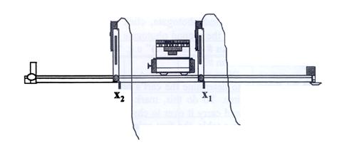
Figure (1) Arrangement of the Photogates
Next, the picket fence is to be placed on the cart and
it is checked whether the photogates are analyzing the cart or not by pushing
it on the track. After plugging the wires of the photogates into the digital
channels 1 and 2, which are on the digital panel of the signal interface as
shown in figure (2). And the interface is turned on by means of the switch at
its back.
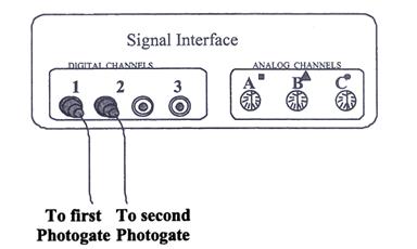
Figure (2) Wire Connections to the Signal
Interface
The computer is turned on by pressing the large button
on top of the keyboard and the “Science Workshop” program started running
automatically. A new file is opened selecting ”New” under the “File” menu and
photogate connections are prepared by carrying the “sensor” logo on the
“digital channel 1” and “digital channel 2” icons and selecting the “picket
fence-photogate”. Then “opaque spacing” is changed settled to 0.01 m by
clicking on the “channel 1” and “channel 2” logos. Doing these, the small cart
is established on the metal track thus the setup became ready for taking data. By
clicking “REC”, and pushing the cart lightly at the same instant, the cart
started its motion. After it passed under the second photogate, “STOP” is
clicked and data labeled as “Run #1” is obtained. In order to get the result,
“Run #1” is marked and “Table” logo is carried over to “channel 1” to have
velocities v1. Finally, it is checked whether there are 12 data
points or not. This step is repeated for “channel 2” for velocities v2
and the whole procedure is repeated twice more for recording data “Run #2” and
“Run #3” similarly.
DATA ANALYSIS
SAMPLE
CALCULATIONS
Data obtained during Run #1 are tabulated in table (1).
|
|
v1 (m/s) |
t1 (s) |
v2 (m/s) |
t2 (m/s) |
|
Run #1 |
0.518 |
2.9381 |
0.505 |
3.3132 |
Table (1)
Sample Calculations for Run #1 are as follows:
Δx = 0.2 m (the separation
between the photogates)
Δt = t2-t1 = 3.3132-2.9381 = 0.375 s
![]() vava =0.5332 m/s
vava =0.5332 m/s
v1+v2 =
0.518+0.505 = 1.023 m/s
![]() vavb =0.5115 m/s
vavb =0.5115 m/s
Δv = v2-v1 = 0.505-0.518 = -0.013 m/s
![]() a = -0.0346 m/s2
a = -0.0346 m/s2
TABLES
Data obtained during the experiment is tabulated in Table (2).
Run #
|
v1 (m/s) |
t1 (s) |
v2 (m/s) |
t2 (m/s) |
|
|
Dv=v2-v1 (m/s) |
Dt=t2-t1 (m/s) |
a=Dv/Dt (m/s2) |
|
1 |
0.518 |
2.9381 |
0.505 |
3.3132 |
0.5332 |
0.5115 |
-0.013 |
0.3751 |
-0.0346 |
|
2 |
0.654 |
2.7432 |
0.641 |
3.0386 |
0.6770 |
0.6475 |
-0.013 |
0.2954 |
-0.0440 |
|
3 |
0.461 |
2.1295 |
0.444 |
2.5540 |
0.4711 |
0.4525 |
-0.017 |
0.4245 |
-0.0400 |
Table (2)
DISCUSSION
QUESTIONS & ANSWERS
(1) After giving a
slight push to the cart, what sort of a motion would you expect from the cart
on an ideal frictionless horizontal track? Explain.
The cart is expected to reach a constant velocity and
then continue moving at the same speed along the same direction from then on. The
average velocity of the cart is will be equal to the instant velocity and the
acceleration will be zero since there is no force acting on the cart during its
motion on the ideal frictionless track.
(2) Considering that
friction exists in reality between the cart and the track, what deviations
would you expect from your answer to question 1?
In fact there exists friction between cart and the
track. As a result, the motion does not
happen as expected. The velocity of the
cart decreases after being pushed since friction acts negatively on the
cart. v2 is then smaller than
v1 and the cart has a negative instant acceleration because ideal
friction is constant on the metal track.
(3) Compare vavea
and vaveb. Do you expect that they will be equal?
Explain.
vavea and vaveb
are expected to be equal since the acceleration should be constant during the
experiment. As we know, vavea
can be equal to average velocity only if acceleration is constant during the
motion because the area under graph of velocity in velocity and time graph of
inconstant accelerating motion is not equal to the area under graph of velocity
in the velocity and time graph of constant accelerating motion.
(4) Do your
results confirm your predictions in questions 1-3? Comment on possible results.
Results do not confirm the predictions completely. For instance, vavea was
supposed to be equal to vaveb, however they did not come
out to be equal since the acceleration was not constant. Also the environment can not be idealized due
to the inconstant friction between the track and the cart, the air resistance
acting on the cart or the rotation of the earth around itself. Additionally experimental
errors may rise during the experiment such as, small measuring errors.
(5) Comment on the
sign of a.
The sign of acceleration came out to be negative for all
3 runs, meaning that the cart is slowing during its motion. Acceleration in
positive direction means that the object is accelerating in the direction of
motion or slowing down opposite to the direction of motion at that time. Acceleration
in negative direction means that object is
slowing down in the direction of motion or accelerating opposite to the direction
of motion.
CONCLUSIONS
During the experiment, the relationship between the
position, velocity and acceleration of an object, moving in one dimension,
along a straight line is investigated. The experiment was carried out under a
condition with a close approximation to ideal frictionless motion (in other
words there is no force acting on the object ideally), and when a constant
force is introduced (gravitational force is acting on the object).
Initial and final velocities of the cart in certain time intervals are measured for 3 different runs. And using the data obtained ,the average velocity of the cart is calculated using two different ways, using equations (2) and (3) mentioned in the theory part. The results obtained were expected to be equal to each other. However they came out to be different since there exists friction between the cart and the track in fact in the real case.
Finally the acceleration of the cart is calculated and found out to be negative, meaning that the cart is slowing down in the positive direction of motion. This acceleration is introduced since the metal track, which assumed to be ideal, is not frictionless in fact and the force acting on the cart is not zero as a consequence.
The results obtained in the experiment are reasonable
but there may be errors due to the misreading of data or inaccuracies in
measurements.